After last week’s post, I thought it might be useful to have some practical examples of how to do sensitivity analysis (SA) of complex models (like climate models) with an emulator. SA is one of those things that everyone wants to do at some point, and I’ll be able to point people here for code examples.

I’ve taken an example from our recent paper that looks at the behaviour of forests in FAMOUS, a low-resolution climate model. FAMOUS model is great because it runs quickly enough that you can create fairly large ensembles, allowing us to build an emulator for the output.

I’ll talk about emulators properly another time, but all you really need to know is that they are statistical models, that simply predict the behaviour of the climate model, when it is run at a particular parameter set. Really, they are just (quite flexible) response functions that allow you to map from input parameters to model outputs, without having to run the model a tedious number of times. Once you’ve run an ensemble suitable for building the emulator, you can replace the climate model with the emulator in any analysis you’d like to do.

Lets assume that you want to do a sensitivity analysis of your climate model. Which of the uncertain input parameters is the climate model output most sensitive to, and how?

You’ll need an ensemble of runs with the parameters of choice varied in some kind of design, and a set of corresponding outputs. The setup is familiar to anyone who has ever done a basic regression analysis. Usually, we designate the design matrix , which has [no. ensemble members] rows and [no. parameters] columns. The corresponding output is a vector of length [ensemble members].

How does variation in affect ?

A quick look

First, plot the model output of interest against each parameter in turn, so we can see if the parameter has any effect at all. In this example, I’ve chosen the average forest fraction in the Amazon region, plotted against each of the seven land surface input parameters that were varied in the ensemble. You can find the details in the paper.

Average broadleaf forest fraction in the Amazon region in an ensemble of FAMOUS, plotted against each parameter in turn.

Pretty useful, but the fact that all of the parameters vary at the same time in the ensemble means that the plots are noisy: the scatter hides the true nature of the relationship between an individual parameter and the model output.

Using the emulator

If the climate model was very cheap to run, we could just vary each parameter one at a time, and then run all of the other analyses that we’d like to do. With an emulator that’s not necessary: we run a single ensemble in a latin hypercube design, build the emulator, and then do all of the analyses we’d like with the emulator.

The downside is that the emulator isn’t perfect. Handily though, it comes with it’s own estimate of it’s imperfection. So below is the one-at-a-time sensitivity plot for the forest fraction in the Amazon forest, along with the 95% confidence interval of the model behaviour.

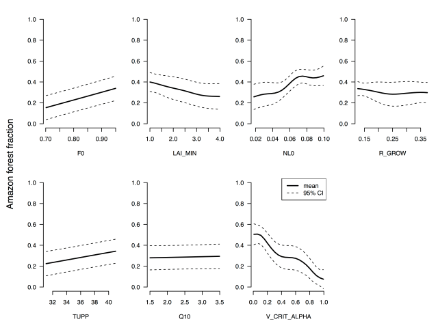
One-at-a-time sensitivity analysis of the average broadleaf forest fraction in the Amazon region in FAMOUS.

We can extend this to comparing the sensitivity of several model parameters to the outputs. Here, I’ve plotted the average forest fraction in the Amazon region against that in the Central African forest (labelled Congo). You can see that the Central African forest is more vigorous across pretty much the entire parameter range. In fact, identifying that the Amazon had too-low forest fraction in the Amazon across the entire parameter set was one of the interesting outcomes in the paper. We offer some ideas for why that might be the case in the discussion.

One-at-a-time sensitivity analysis using the emulator. Average broadleaf forest fraction in FAMOUS in the Amazon is shown in black, and Central African region is green, with shaded areas representing the 95% CI.

Technical notes

I’ve used the DiceKriging package in R for a Gaussian process emulator. You can view the code here.

I’ve used the km() function pretty much out-of-the-box to build the emulator for clarity, but finding the best emulator and verifying that it works is another blog post. Similarly, I’ve not messed around with the base R graphics too much.

The corresponding plot for all of the forests can be found in the paper, figure 6. We also use the R sensitivity package and the fast99 algorithm to do some sensitivity analysis, but again that is another blog post.

Paper: The impact of structural error on parameter constraint in a climate model | D. McNeall et al. Earth Syst. Dynam., 7, 917-935, 2016