This post is an introduction to our new paper, The potential of an observational data set for calibration of a computationally expensive computer model, for non specialists. The paper is in open review, and so can be commented on by anybody. We would appreciate feedback, so please consider making a comment at the open review by 4th June 2013.

What is the paper about?

The paper describes a method for working out how much a new observation (say, from a new satellite or ocean observing array, for example) might help us to constrain* the projections of a climate model. The projections are plausible realisations of paths that the climate might take in the future. We’d like to distinguish plausible projections from implausible ones.

What is the big idea?

The nub of the idea is that we can use data from the climate model, as if it were an observation of the real world. We can use this simulated world to get an idea about how much information an observation would give us about our climate model in the best possible case. Of course, in the real world, we won’t get as much information from our observations, as they have uncertainty, and we know that our model doesn’t perfectly match reality. Our paper also proposes a framework for understanding how much information we lose because of those uncertainties.

This sort of perfect model experiment is fairly common in climate science and in the world of computer experiments. We’ve used some techniques that help when our climate model is very expensive – that is, we can only afford the computer time to run a few (or a few tens or hundreds) of simulations. We’ve also applied our techniques to a real model of part of the climate system – one that represents the Greenland Ice sheet.

What’s the setup?

Climate models are mathematical representations of the real world that attempt to reproduce important physical relationships in the climate system, inside a computer. They often contain simplifications of some of those processes, called parameterisations. These simplifications are usually there because the model is computationally expensive – that is, running a simulation takes a lot of computing power or time. Sometimes the parameterisations are there because the exact physical relationships are not very well known.

Parameterisations in simulators usually have associated constants (we’ll call them parameters); numbers that may or may not have some physical analogue in the real world. We have uncertainty about the best values of these constants, those that mean that the behaviour of the climate model best matches that of the real world.

This parameterisation uncertainty, along with errors in our understanding, and unknown future forcing factors (such as the amount of CO₂ we’ll emit), introduce uncertainty in our predictions about the future behaviour of the climate.

We’d like to be able to choose a good set of those input parameters – to constrain them by comparing our climate model output with observations of the real world.

Visualising the problem

It can be helpful to think of the climate model as a function that maps a set of uncertain inputs (parameters, forcings), to a set of climate states – for example temperatures and precipitation in the model.

Different points in the input space defined by the inputs map to different climate states – points in the output space. If we run a collection of simulations, at different points in the input space, we end up with a collection, or ensemble of climate simulations. If we pretend for the moment that we had a perfect model of the climate system, mapping the ensemble would look like this.

Figure 1. An ensemble of climate model simulations. A point in the input space is defined by the value for forcing (F) and parameter (λ). These points map to the output space of temperature (T) and precipitation (P), through the climate model g(.).

Some of these ensemble members will be more realistic than others. If we were to make an observation of the state of the real world, we could compare it with the output of the ensemble, and only keep those ensemble members that looked the most like the real world. Of course, we’d have to make some judgements about how close to the real world we want the ensemble members to be – we have some uncertainty about the observations, after all. Members of the ensemble that were too far away from the real world could be regarded as “implausible”, and the corresponding inputs ruled out as representing reality.

Figure 2. Observation uncertainty implies input uncertainty. If an observation falls within the red rings in output space, this implies a plausible region of input space.

A good measure of the ability of the observation to constrain the model is the size of the region of input space that is still plausible, relative to the original input space.

We can take the inputs that we haven’t ruled out yet, and run them through the climate model, simulating the future. This gives us a constrained set of plausible projections of future climate.

Figure 3. Projections of future climate can be constrained by matching the output of the model to historical observations, and projecting forward the resulting regions of input space. Here, g_f(.) is the climate model that represents future climate processes.

Another good measure of the ability of the observation to constrain the data is the size of the future  output space that is not ruled out by the data.

Emulators

The problem that we have with the above setup is that the number of simulations that we need to run can become very large indeed. We’ve depicted input space and output space as having only two factors – or dimensions. In reality, both spaces might have tens, hundreds, or (if we’re really unlucky), even thousands of dimensions. It is difficult to explore all of the uncertainties with only a few climate model runs, due to something called the curse of dimensionality.

Luckily, we can break the curse by using a few assumptions, and some statistical methods. Assuming that the climate model doesn’t behave in really unpredictable ways, we can build an emulator. This is a cheap-to-compute statistical approximation of the climate model, made possible by running a special type of ensemble, specifically designed to explore uncertainties. The emulator is typically many thousands of times cheaper and faster to run than a full climate model.

The emulator predicts the output of the climate model, at any combination of inputs. There is no such thing as a free lunch, however and the emulator isn’t perfect! As a statistical model, the emulator contains an estimate of it’s own uncertainty.

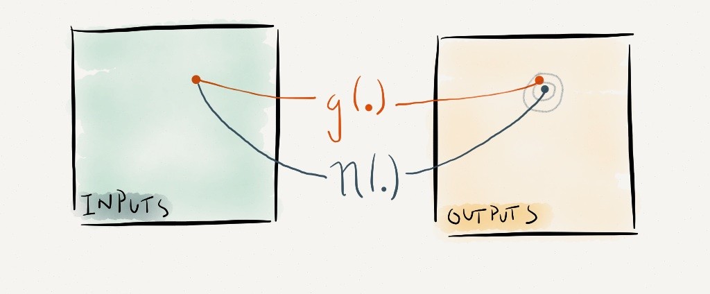
Figure 4. An emulator η(.) is a statistical model that predicts the output of a climate model, at any set of inputs. The emulator needs an ensemble of example model simulations, in order to train it.

Once you’ve built the emulator, you can use it to do almost any experiment that you can think of, that you might have otherwise done with the climate model. It replaces the climate model in our mapping diagram.

We’d like to invert the emulator, and find a good set of input parameters, given an observation. We’ll need to include all of the uncertainties, in order to find that good set of inputs.

Including all of the uncertainties

For simplicity, we’ve skipped over some important sources of uncertainty when we’re relating our problem in the world of the climate model, to the real system.

Here is a list of all list  the uncertainties that that need to be taken into account when we estimate how useful our observations are for constraining the parameters of the climate model. In our experiment, we treat them all in a similar way, in that they each affect the plausibility that a point in input parameter space might be the ‘best’ input.

1. Uncertainty in the observations – perhaps we only have a short record, or there may be biases in our observation system.
2. Model discrepancy uncertainty – this is our uncertainty about the difference between the climate model and reality. This needs to be taken into account at the same time as the observational uncertainty.
3. Emulator uncertainty – due to the fact that the emulator and the climate model are not the same. We can’t run the climate model at every point in input space, and so our approximation – the emulator – has it’s own uncertainty.

Including all of these uncertainties, the mapping of observations to input parameters and future projections now looks like this:

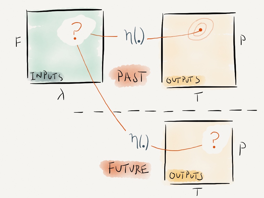
Figure 5. Replacing the climate model with an emulator, and including model discrepancy when projecting future climate.

Cross validation

Now we have all the elements we need to run our experiment, to find out how, in the best possible case, a new observation might constrain our climate model.The trick is to use each ensemble member in turn as a pseudo-observation, and then to see how well that pseudo-observation constrains the climate model.

Here is the sequence;

1. Run an ensemble of climate models, with plausible values for the input parameters.
2. Hide one of the ensemble members from view. Build an emulator using all of the other ensemble members.
3. Now, pretend that the output from the hidden ensemble member was an observation of the climate. Use the emulator to estimate the (hidden) input parameters of the ensemble member.
4. Measure how well you can estimate those parameters – how big is the input space that isn’t ruled out as implausible?
5. Repeat for all of the ensemble members!

We’ll end up with a collection of estimates of the amount that we can constrain the climate model, that depends on the precise value of the pseudo-observation. If we repeat the analysis with different outputs we can compare them, and see which one might help us constrain the model the most. This could help us prioritise observations to make in the real world.

Going further

So far we’ve imagined that the climate model is a perfect representation of the true climate, and the observation is perfect. This is the best possible case, but is unrealistic.

Our experiment setup allows us to simulate a more realistic situation. We can add in as much simulated uncertainty into the pseudo-observation as we like, and also pretend that we have more uncertainty about the the climate model than we really do. In doing so, we can test how those uncertainties reduce our ability to constrain the climate model.

Our results

We used an ensemble of the ice sheet model Glimmer in order to test the method. We had 250 ensemble members, with 5 uncertain input parameters, and a single output parameter (ice sheet thickness). The output was the thickness of the ice sheet over all of Greenland. Because we had the output data on a grid, We could organise it in three slightly different ways: 1) total volume, 2) surface area and 3) maximum thickness.

We found that:

1) The different ways of organising the data gave you different amounts of constraint, on different input parameters. For instance, maximum ice thickness was really useful for constraining one of the input parameters. Ice volume was the best all-rounder.

2) Adding even a little bit of uncertainty to the psuedo-observations really diminished our ability to constrain the input parameters.

3) Using all three of the outputs at once to constrain the inputs got us back towards a useful level of constraint, even when there was observational uncertainty.

Next steps

We’d like to use our method to help identify the best ways to constrain our future projections of climate change. This might mean helping identify which are the most useful observations that we’ve made in the past, or it might suggest new observations that we could make in the future.

UPDATE 17/04/2013

Mat Collins (@mat_collins) points out that the diagrams in this post are structurally similar to those in his paper Quantifying future climate change (preprint version). I’d recommend the paper – I read it when it came out, and so the similarities are probably no coincidence ;).

Notes

* We use constraint, but calibration, tuning, data assimilation and solving the inverse problem could also be used here. This kind of problem has been tackled in many different ways, and in many different fields. This is one of the reasons that writing an introduction to the paper felt hard.

This work is built upon a huge amount of work by other people. Please check the paper for the appropriate references – and let us know if we’ve missed any really important ones. Preferably via the online interactive discussion at GMDD, by June 4th 2013.

The paper authors would like to Thank to Ed Hawkins for comments on a previous version of this blog post.

McNeall, D. J., Challenor, P. G., Gattiker, J. R., and Stone, E. J.: The potential of an observational data set for calibration of a computationally expensive computer model, Geosci. Model Dev. Discuss., 6, 2369-2401, doi:10.5194/gmdd-6-2369-2013, 2013.